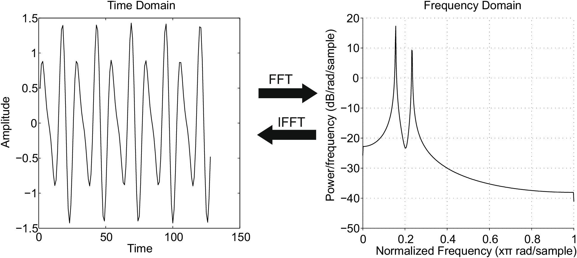
Measurements and Data Analysis for Agricultural Engineers using Python

7.1 Time and frequency domain

The interesting information in a signal can be found from frequency domain or time domain, or we can be interested in both. The information in time domain describes when something occurs and what the amplitude of the occurrence is. e.g. milk flow rate in different stages of milking, air humidity coming from a grain dryer.

The information in frequency domain is periodic, it describes how often something happens. Typical frequency domain signals are sound, vibration and respiration.

Time domain : signals are indexed by time ¹ .
Frequency domain : signals are indexed by frequency.
FFT Fast Fourier transform is used to change signal from one domain to another.

Time and frequency domain representation of a signal.

7.2 Discrete Fourier Transform

Discrete Fourier Transform (DFT) is used to transform a signal from time domain to frequency domain. That is calculating the frequency components from time series data. The result of the transform is called the spectrum or power spectral density PSD of the signal.

DFT is a nonparametric method for estimating the spectrum i.e. it doesn’t assume that the data follows a specific model and is a fairly robust method. Autoregressive models are parametric methods for spectral estimation and they have more strict assumption about the data.

Fast Fourier Transform FFT is computationally efficient algorithm to compute DFT.
In practice the two terms are often used interchangeably.
DFT works by fitting sine and cosine waves of different frequencies to the time series data. The correlation between the sine and cosine wave of specific frequency then becomes the value of that frequency in the frequency spectrum.

DFT \( X_k \) for time series \( x_n \) is defined as:

\begin{align} X_k = \frac{1}{N}\sum_{t=0}^{N-1} x_n \cdot e^{-i 2 \pi \frac{k}{N} n} \end{align}

where \( k = 0,1 \dots \frac{N}{2} \)

This is the complex form of the transform, but it can also be expressed in friendlier form using familiar sines and cosines (Real DFT):

\begin{align} ReX_k = \frac{2}{N} \sum_{n=0}^{N-1} x_n \cdot cos(2 \pi \frac{k}{N} n) \end{align}

\begin{align} ImX_k = \frac{-2}{N} \sum_{n=0}^{N-1} x_n \cdot sin(2 \pi \frac{k}{N} n) \end{align}

And the magnitude is:

\begin{align} MagX_k = \sqrt{ReX_k^2 + ImX_k^2} \end{align}

The power spectral density (PSD) \( S_k \) is calculated as in (Percival & Walden 1998):

\begin{align} S_k = \frac{MagX_{k}^2}{2} \end{align}

By definition the sum of elements in PSD equal the sample variance \( S_k \equiv \sigma^2 \) , (Percival & Walden 1998) that is:

\begin{equation} \label{eq:denvar} \sum_{j=1}^{k} S_k = \sigma^2 \end{equation}

The spectrum is calculated for fundamental frequencies [spectrum4]. The frequency resolution of the spectrum depends on the number samples used in the Transform and the sampling rate and is given by: \( \frac{\text{Sampling rate}}{N} \) . The computation of Real the real DFT is explained in (Smith 1997) Ch.8 and the complex DFT in Ch. 31.

7.3 Practical DFT using FFT in Python

The good news is that you don’t need to write the equation to the computer, but they have already been implemented for you in most software packages. This means you can use it easily when you remember certain basic principles.

Software usually returns the complex version of FFT and therefore you need to use absolute values of the result when you plot the frequency spectrum.
The length of the signal must be power of 2 so \( 2^n \) (256, 512, 1024) for most FFT implementations, but a lot of software takes care of this automatically by truncating or zero padding the data.

You can use scipy.signal.periodogram to get the power spectrum and power spectral density and pyageng.pfft to plot it.

Have a look at an example:

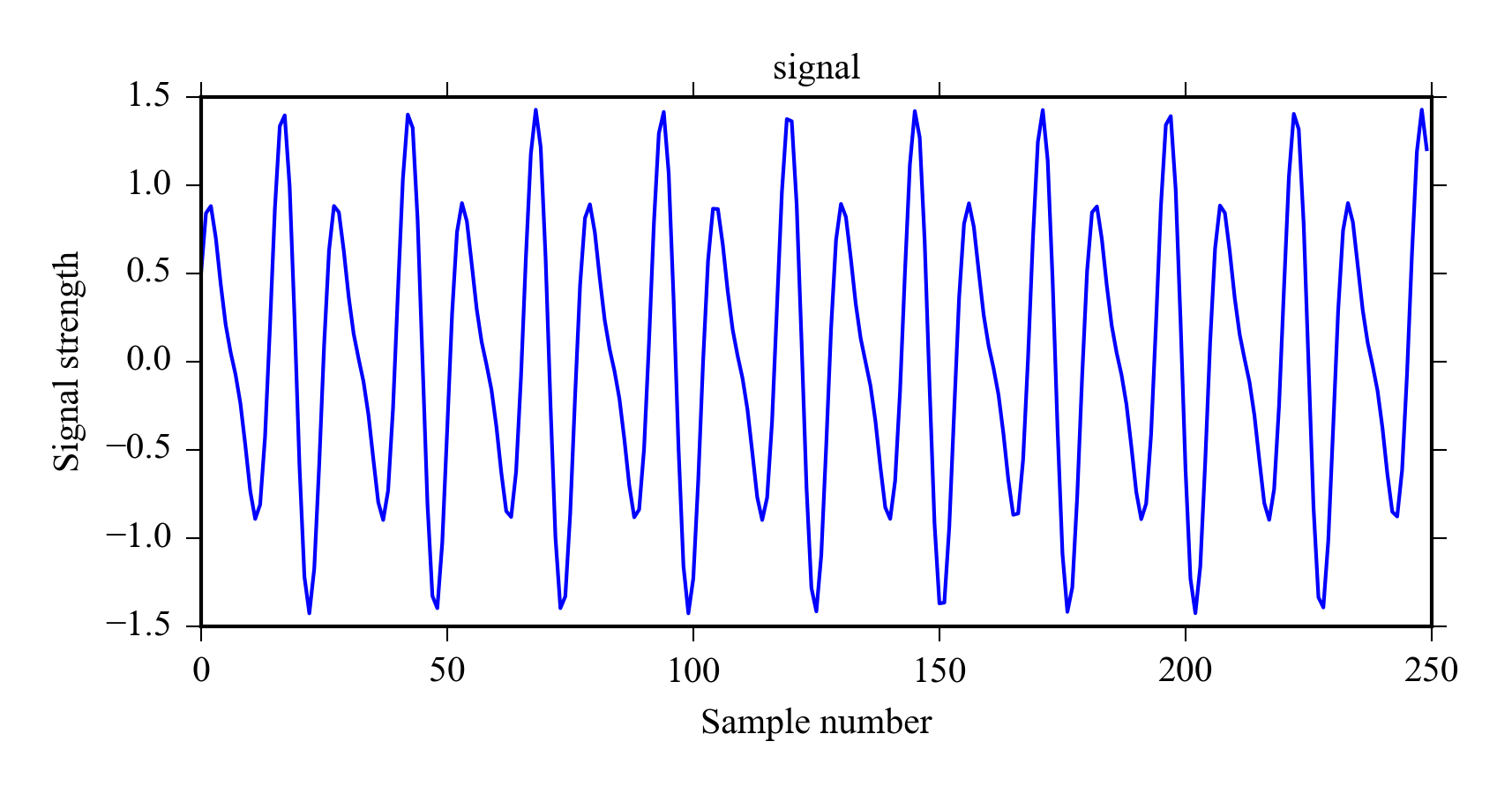
Let’s first create a signal with two frequency components.

from pylab import *
#Create a signal
x = sin(linspace(0., 500, 1024)) + 0.5*cos(linspace(0, 750, 1024))
plot((x)[0:250])
title('signal')
ylabel('Signal strength')
xlabel('Sample number')

We will calculate \( S_k \) for frequencies \( f \) using scipy.signal.periodogram . The scaling is set to “density” by default in which case the returned spectra is returned in units magnitude / frequency we set it to spectrum to verify equation 7.6 . Setting return_onesided to true returns only the first half of FFT in real numbers, which usually what we are interested in.

The function accepts the same arguments as scipy.signal.periodogram .

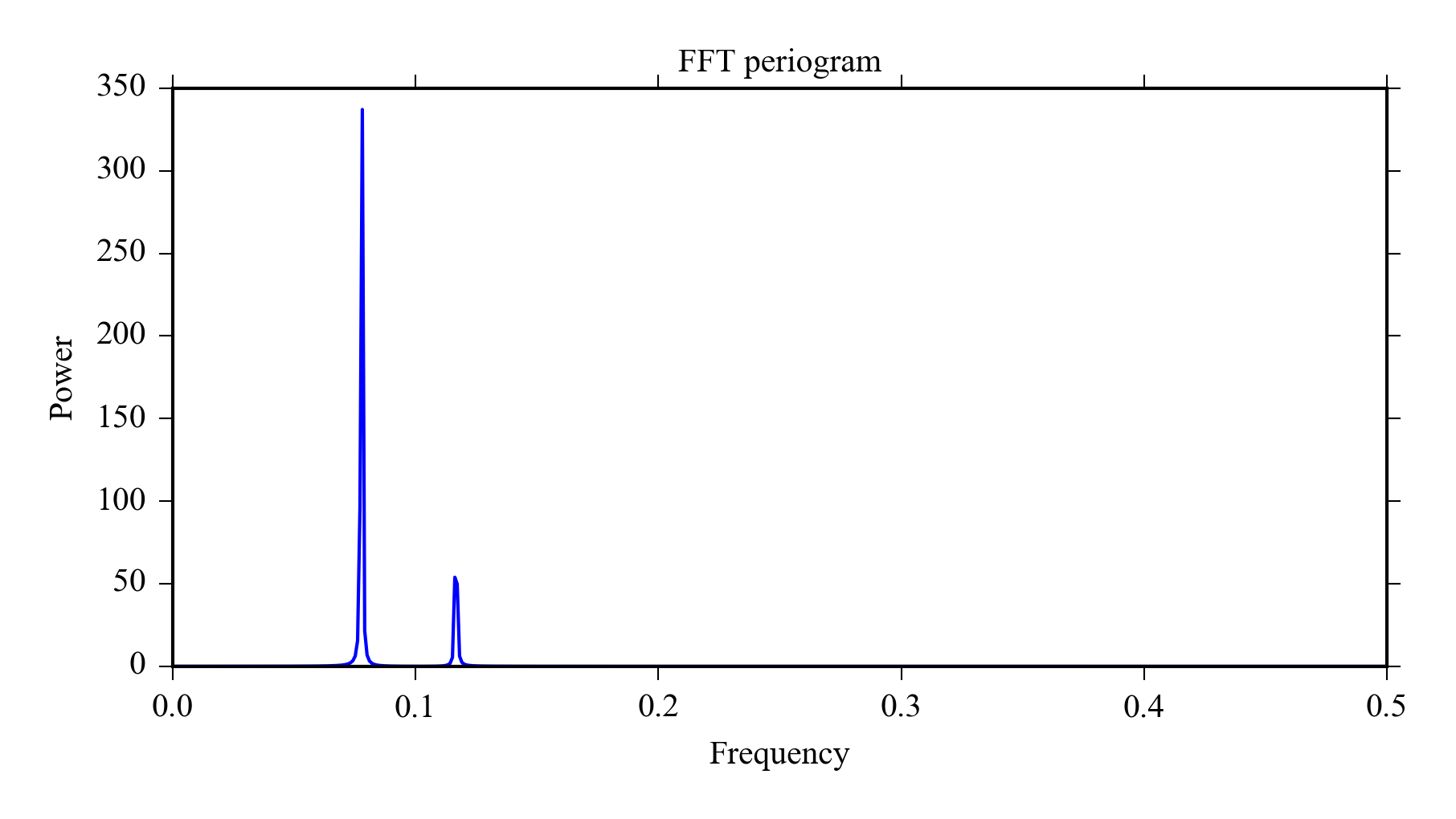
>>> from scipy import signal
>>> f, Sk = signal.periodogram(x, nfft = 1024, return_onesided = True,
scaling = "spectrum")
>>> # Check that sum(Sk) equals variance of x
>>> sum(Sk) == var(x)
True

Finally we use pyageng.pfft the to plot the periodogram, this time using the default scaling. The plot shows that main frequencies contained in the signal are around 0.08 and 0.12, the unit is relative to sampling rate.

import pyageng
pyageng.pfft(x)

7.3.1 FFT pitfalls

There are certain common pitfalls for people new to DFT/FFT. Sometimes you can see a clear period in the data, but nothing in the spectrum this is usually because the data needs to have a zero mean and can’t have any linear trends for FFT to behave nicely. Another common mistake is to try to improve the resolution by increasing sampling rate which also doesn’t work, you need to increase the sampling time to get better resolution.

Here is a checklist to successful FFT:

You need to remove the mean and linear components from data before computing FFT.
The biggest frequency in spectrum is half of the sampling rate.
The frequency resolution of the spectrum depends on the duration of the sample.
The transform assumes that the signal is stationary (=the frequency doesn’t change)

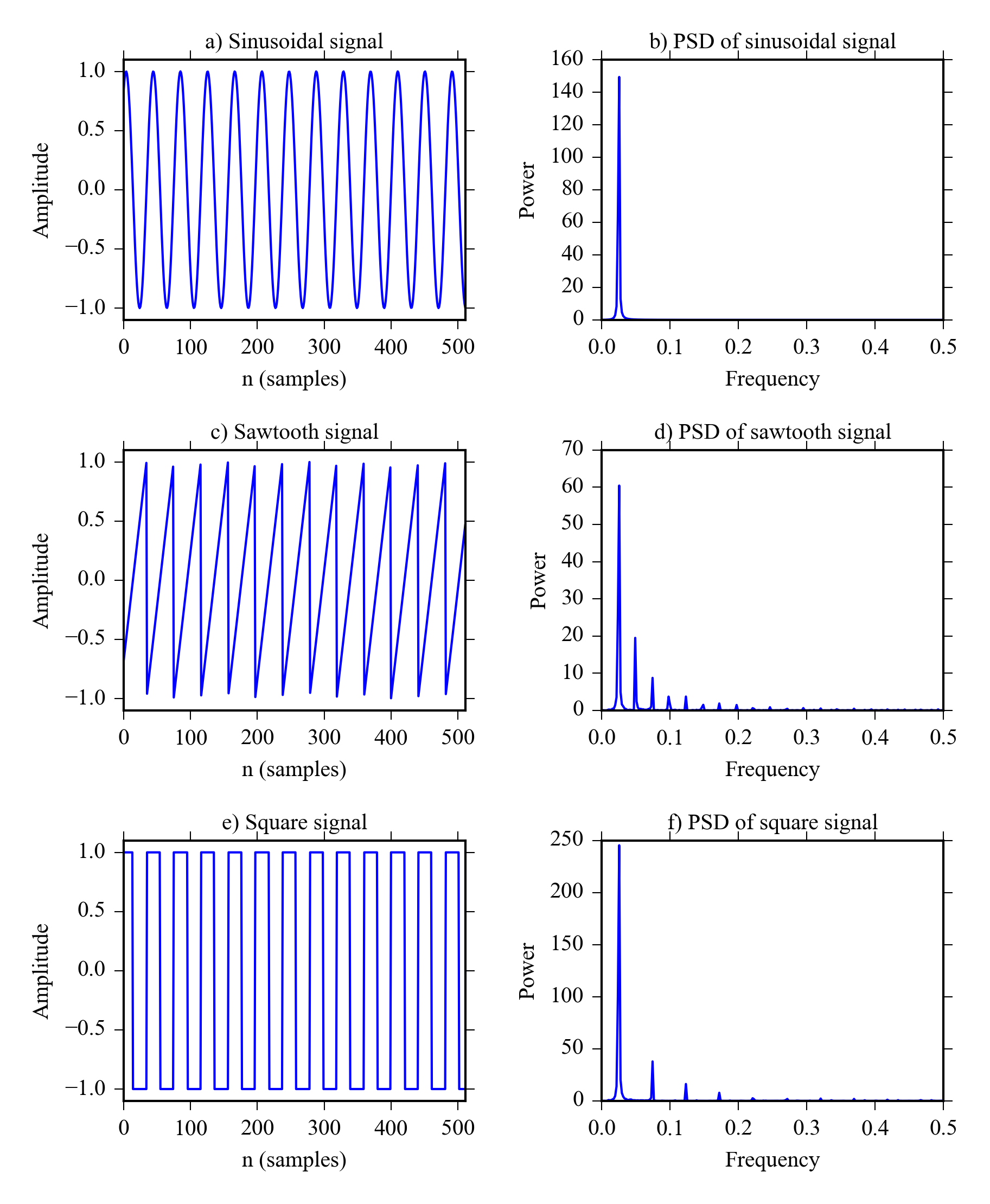
7.3.2 Harmonics

Harmonic waves are are integer multiples ( \( 2\cdot f, 3\cdot f, \dots \) ) of the fundamental frequencies so e.g. the fundamental frequency of 1Hz has harmonics in 2Hz, 3Hz and so on.

DFT is calculated only for fundamental frequencies. This means that each sine and cosine wave used to calculate the power of a frequency is uncorrelated with others and no exact harmonics are used in the transform. In practice this means that there is only one peak in the PSD for a perfect sine wave ( Figure 7.2 a and b).

However real world signals are usually not perfect sinewaves, they have a different shape and their frequency fluctuates. Because the fundamental frequencies used in DFT are very close to each other it means that multiple peaks can be seen in PSD for non-sine wave periodic signals.

The PSD of sawtooth wave in Figure 7.2 c has the highest peak at its actual (normalized) frequency 0.025, the second peak at 0.049 and the third at 0.074. While these are not exact harmonics they are very close and you often see these peaks appearing when you used DFT for actual measured signals.

It is worth noting that the sawtooth and square waves actual contains multiple different frequencies because their rate of change varies. The sawtooth has a higher frequency when it falls than when it rises and the square wave has high frequency when it rises and falls, but zero frequency at the top and bottom.

Here is the code used to make Figure 7.2 :

from scipy import signal
from pylab import *
x = linspace(1, 80, 512)
from pyageng import *

def plot_signal(x):
    plot(x)
    axis('tight')
    ylim(-1.1, 1.1)
    xlabel('n (samples)')
    ylabel('Amplitude')

figure(figsize=(6.5,8))
subplot(321)
sx = sin(x)
plot_signal(sx)
title("a) Sinusoidal signal")
subplot(322)
pfft(sx)
title("b) PSD of sinusoidal signal")

subplot(323)
sax = signal.sawtooth(x)
plot_signal(sax)
title("c) Sawtooth signal")
subplot(324)
pfft(sax)
title("d) PSD of sawtooth signal")

sqx = signal.square(x)
subplot(325)
plot_signal(sqx)
title("e) Square signal")
subplot(326)
pfft(sqx)
title("f) PSD of square signal")

#Add space between subplots
subplots_adjust(hspace=0.5, wspace=0.4)

savefig('images/DSP/harmonics.png')

DFT from sine wave, sawtooth and square wave of the same frequency. Notice that the PSD of sawtooth and square wave also show the harmonics of the frequencies. The power is shown in linear scale.

7.4 Welch Transform - spectral averaging

Welch’s Method to calculate PSD uses averaged overlapping FFTs resulting in smoother estimates.

Can be calculated using e.g. 50% overlap.
Can use windowing resulting in smoother spectra.
Decreases resolution, but gives cleaner PSD.
Especially useful if you are only interested in the main frequency component (=highest peak).
scipy.signal.welch command in Python and pyageng.pwelch for plotting.

7.5 Autoregressive models

Autoregressive models assume that each datapoint in a timeseries ( \( x_t \) ) can obtained with regression of \( n \) previous values ( \( x_{t-1}\ldots x_{t-p} \) )

They can be estimated using several different methods: Least squares, Yule-walker and Burg.
The model order p is usually chosen using some information criteria: BIC or AIC.

Autoregressive model of order p, AR(p) for time series \( x_t \) is given by:

\begin{align} x_t = \phi_1 x_{t-1} + \ldots + \phi_p x_{t-p} + \epsilon_t \end{align}

where \( \epsilon_t \) is white noise and \( \phi_1 \ldots \phi_p \) are model coefficients.

AIC (Akaike information criteria) is a measure of relative goodness of fit and it is used to find the best model. It tries to choose the optimal number of parameters and avoid overfitting by finding a balance between goodness of fit and the number of parameters. AIC is calculated using:

\begin{align} \text{AIC} = 2k - 2\text{ln}(L) \end{align}

where k is the number of parameters and L is the maximized likelihood of the fitted model.

7.6 Fitting AR models

7.6.1 Least squares with direct inversion

Due to the fact that AR model of order \( p \) can be viewed as regression of \( p \) previous values you can fit them using ordinary least squares as you would fit a regular regression model.

Suppose we want to fit an AR(3) model to series \( x_t \) with \( N \) elements. We can form an overdetermined system:

\begin{align} \mathbf b = \mathbf A \mathbf \phi \end{align}

where the matrices are:

\begin{align} \begin{pmatrix} x_4\\ x_5\\ \vdots\\ x_N \end{pmatrix} = \begin{pmatrix} x_3 & x_2 & x_1 \\ x_4 & x_3 & x_2 \\ \vdots & \vdots & \vdots\\ x_{N-1} & x_{N-1} & x_{N-3} \end{pmatrix} \begin{pmatrix} \phi_1\\ \phi_2\\ \phi_3 \end{pmatrix} \end{align}

We can then solve the AR coefficients \( \phi \) using least squares estimator:

\begin{align} \Phi = (A^\intercal A)^{-1}A^\intercal b \end{align}

This is exactly the same method that is used for linear regression models and it is fairly easy to implement using SciPy, but it is not very computationally efficient if you have a lot of data.

7.6.2 Yule-Walker method

First we need to compute autocorrelation function \( r_t \) Then we can form Yule-Walker equations:

\begin{align} \mathbf r = \mathbf R \Phi \end{align}

\begin{align} \begin{pmatrix} r_1\\ r_2\\ \vdots\\ r_p \end{pmatrix} &= \begin{pmatrix} r_0 & r_1 & \ldots & r_{p-1} \\ r_1 & r_0 & \ldots & r_{p-2} \\ \vdots & \vdots & \ddots & \vdots \\ r_{p-1} & r_{p-2} & \ldots & r_0 \end{pmatrix} \begin{pmatrix} \phi_1\\ \phi_2\\ \vdots\\ \phi_{p}\\ \end{pmatrix} \end{align}

The parameters \( \phi \) can then be solved directly using:

\[ \Phi = \mathbf {R}^{-1}r \]

7.6.3 Power spectral density with AR models

Spectrum is calculated parametrically from the model parameters.
AR spectrum should only be used if the resolution of FFT is not sufficient i.e. for short samples.
The model order affects the result significantly so it needs to be chosen carefully.
The spectral estimates might be completely wrong if the model doesn’t fit to the data well.
Use detrending and filters when needed.

Even though AR models are usually not the preferred method for frequency estimation they are extremely useful otherwise. AR models are frequently used in time series analysis and forecasting, they are also used with good results in model based control. Madsen (2008) is a good reference for AR models and time series analysis.

7.6.4 AR spectrum using Python

A small python example (see pyageng -module source for implementation).

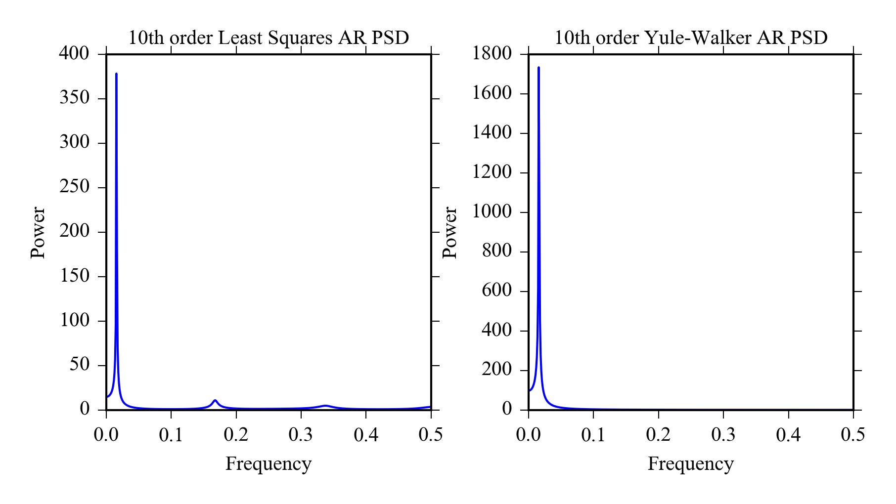
x = sin(linspace(0, 50, 500))
from pyageng import *
subplot(121)
pcov(x) #Least squares estimate
subplot(122)
pyulear(x) #Yule-Walker estimate

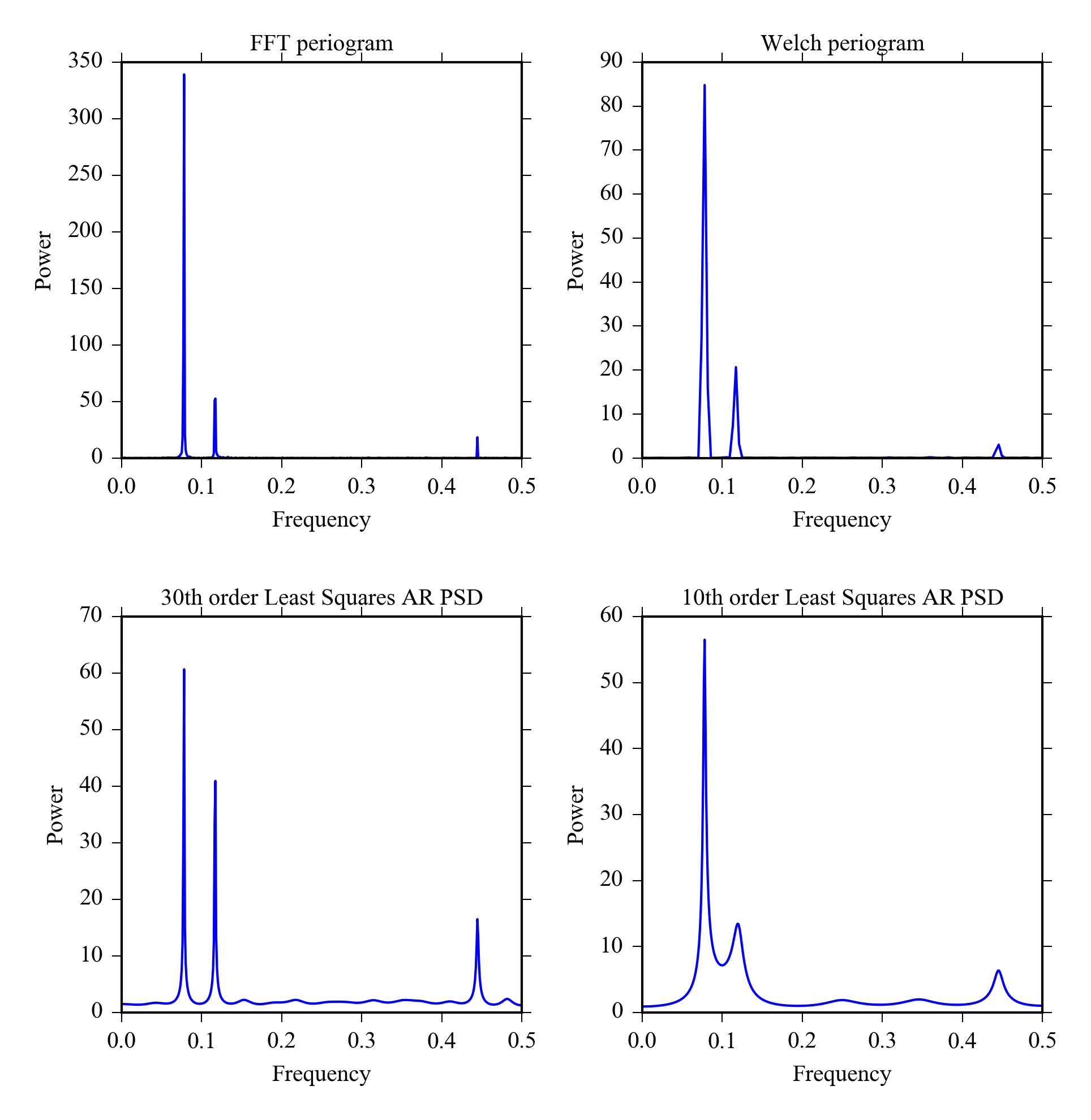
7.7 Comparison of FFT, Welch and AR

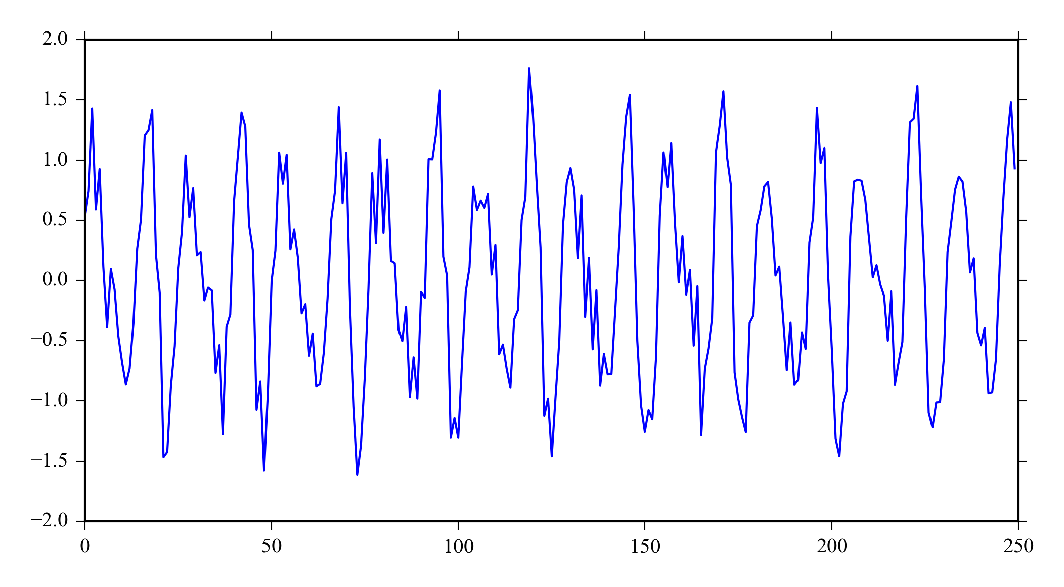
Figure 7.3 shows a signal that has two frequencies of interest with random and high frequency noise. Notice that you can’t tell that some of the noise is frequency specific from the time series data, but there is high frequency peak in the signal spectra ( Figure 7.4 ). The signal is generated with Python using.

x = sin(linspace(0, 500, 1024)) + 0.5*cos(linspace(0, 750, 1024)) + \
      randn(1024)*0.2 + 0.2*cos(linspace(0, 10000, 1024))

plot(x[:250])

A generated signal with two frequency components and added noise.

We will calculate the PSD using the different methods and plot them in one figure:

subplot(221)
pyageng.pfft(x)
subplot(222)
pyageng.pwelch(x, nfft = 256, noverlap = 128)
subplot(223)
pyageng.pcov(x, 30)
subplot(224)
pyageng.pcov(x, 10)

PSD estimates of signal from Figure 7.3 with different methods. Units are y-axis: Power/frequency; x-axis: Normalized frequency

7.8 Exercises

How do you convert a signal from time domain to frequency domain?
When would you use autoregressive model for PSD estimation? How do you choose the correct order of the model?