1.1 Why do we measure things?
Measurements form the basis of empirical research. The purpose of measurements are usually divided in the following three categories:
- Observe a process : Home temperature, electricity consumption, water consumption, CO level in garage, medical diagnostics. Not actually research and not (at least automatic) control.
- Research : Test theories with measurements (testing a model for plant growth), create experimental models for a relationship between factors for phenomena with no existing theory (predict cattle lameness based on weight distribution during milking).
- Control : we want to automatically control a process given certain parameters. e.g. control the fan speed and inlet openings of a barn based on temperature and \( CO_2 \) measurements.
Fault diagnostics is one popular application of measurements based on observing a process. A machine, animal or a plant is monitored with a sensor and model predicts when there is a failure or disease. E.g the lameness in cattle can be predicted using force sensors, pig cough can be measured using sound analysis and bearing failure in machinery can predicted based on resonance frequency. The models used to predict problems can be very simple based on limit values or more complex models that are fitted to data based on sample dataset(This is called machine learning).
The objectives can also overlap e.g. we may want to also research the process we are controlling. The purpose of the measurement affects its requirements for accuracy and reliability.
1.2 The phases of a successful measurement
1.2.1 Planning
Plan the measurements carefully. Incomplete planning will compromise the whole study. Ask the following questions when planning:
- What things affect the measured quantity? Can you measure or control these variables?
- What is the rate of change of the measured phenomenon? What is the suitable sampling rate?
- What is the required accuracy and precision of the measurement? This together with the sampling rate will determine the needed measurement system.
-
How are you going to store the data?
Which format will be the best
for further processing?
How to make
backups? - The placement of sensors so that you minimize interference to signals and the effect to the measurement system to the measured system.
- Measurement location if you’re taking samples.
These notes try to give you means for answering all of these questions.
1.2.2 Preparing
- Build the entire measurement system and make sure you know how to use it. Practise!
- Write the software and check that it is working.
- Make a pilot study and analyze the results to make sure the system is working as expected. Revise if needed!
- Calibrate the system.
- Make a measurement plan with locations and schedule.
- Make notes of the circuit you’re using, calibration procedure and calibration coefficients. Make sure you have notes of all parameters used in the system.
- Make sure you have all necessary equipment and spares.
- Plan how the calibration and performance of the system will be followed during long measurements.
1.2.3 Executing
- Follow the plan. If you need to make changes, write everything down.
- Make exact notes of how the measurements were executed with exact times. Add everything that you think might have an effect.
- Make sure that the system is working during the measurements. If possible make the software to plot the results continuously or a LCD screen showing measured values etc.
- Check the performance and calibration of the system according to your plan.
1.2.4 Analysis
- Try to analyze the results as soon as possible after the measurement. This way you’ll still remember what happened in case your notes are incomplete and its more likely you can still make more measurements if needed.
- If the measurement is running over several months or years make preliminary analysis when the experiment is still running. It is common that you have to return back to planning or collect more data after initial analysis.
1.3 Measurement system components

Sensor is a transducer that convert a physical quantity to a measurable analog signal.
ADC (analog-to-digital converter) converts the analog signal to digital
A computer/datalogger/microcontroller is used to store and display the information.
The wires from sensor to ADC should be as short as possible to minimize noise and level changes. Voltage signals suffer from voltage drop when long wires are used due to the resistance of the circuit. Current signals however are a lot less sensitive to interference and don’t have a problem with level changes.
Digital signals can be transmitted without a loss of information with efficient compression (e.g. using the Internet) and are therefore the preferred method for transmitting data.
1.4 Signals
A signal is a description of how one parameter relates to another. Usually signals are measured as a function of time e.g. how temperature changes over time, however they can be also measured as function of e.g. distance or light intensity.
1.4.1 Analog signals
Analog signals : (voltage, current) take continuous range of values. Most real world signals are continuous.
- Commonly used analog signals are voltage signals (0-10V, 0-5V etc.) or current signals (4-20mA)
- Analog signals are converted to digital signals using sampling and quantization i.e. Analog-to-Digital(AD) conversion.
1.4.2 Digital signals
Digital signals are discrete, they can only take limited range of values and are sampled at a certain interval. With proper sampling the digital signal can represent all the information present in the original analog signal.
The quality of the sample depends on the accuracy of the AD conversion and the sampling rate .
Computers can only work with digital signals and they have numerous advantages over analog signals:
- They can be compressed efficiently
- Efficient storage and data transfer
- Several digital signals can be transmitted in the same wire or radio channel.
- Digital signal processing allows the use of more sophisticated filters.
Some digital signals such as the one in USB cable are still voltage signals, but they only take two levels representing binary values 0 and 1. Digital signals are also commonly transferred wirelessly or in optical fibres.
1.5 Analog to digital conversion
Analog-to-digital converterss ( ADC ) work by taking a sample of the original signal and comparing it to a fixed number of known voltage levels. The signal is then rounded to the closest reference level. The resolution of the ADC is given in bits which means that the number of values the digitize signal can get, for \( n \) bit ADC is \( 2^n \) . Each ADC works for a certain voltage range e.g. 0 – 5 V.
- Taking a sample of analog signal for digitization is called the sample-and-hold method.
- Analog signal is rounded to the nearest possible value. The difference between the original value and the digitized sample is called quantization error .
- The difference between adjacent conversion levels is called least significant bit (LSB)
- The maximum quantization error is therefore \( \pm\frac{1}{2} \) LSB.
Suppose we have an 8bit ADC with the range of 0-5V. It can produce \( 2^8 = 256 \) distinct numbers (0-255) so with the range of 5V its voltage resolution is 5/256 \( \approx \) 20 mV. This value is also called LSB .
This means in practice that when digitized analog values 10 – 30 mV are rounded to 20mV and analog values 30 – 50 mV to 40mV etc. The quantization error for analog value 10mV is 20mV - 10mV = \( \frac{1}{2} \) LSB.
Now if you have a temperature sensor with the sensitivity of \( \frac{10mV}{^{\circ}C} \) . then digitization introduces an error of \( \pm 1^{\circ}C \) to the measurement. If you want to increase the precision of your measurement you need to use an ADC with higher resolution . This still doesn’t guarantee that the measurements will be accurate , for that you need calibration .
The voltage resolution of the ADC can be calculated with:
So the voltage resolution for 12bit ADC with -10 – 10V range is:
| Bits | Levels | mV |
| 8 | 256 | 20 |
| 10 | 1024 | 4.9 |
| 12 | 4096 | 1.2 |
| 14 | 16 384 | 0.3 |
| 16 | 65 536 | 0.08 |
The number of values we get an ADC determines how accurately we can measure things in a certain range. We can get the best accuracy when use the whole voltage range of the instrument. Usually we need to scale the signal either by amplifying or reduce the original signal to achieve this.
We’ll learn some options for reducing the signals amplitude in the exercise. If you need to amplify a signal you can use operational amplifiers, we are not doing that in the course but you can find the needed circuits from basic electronics books. There are also special amplifiers for common small signals e.g. for load cells and thermocouples.
ADC resolution fixes either the range or accuracy of your measurement. Suppose you have a scale with 10bit resolution. If you want to measure weight with 1g accuracy it means that the maximum range you can have is 1024g.
Or if you want to use the same ADC to weigh 10 000 kg of grains the maximum resolution you can get is 10 kg. If you need either wider range or better accuracy you’ll need to use a device with higher resolution.
1.6 Sampling
In addition to getting accurate samples of the voltage we also need to consider the rate of change of the signal. Here are two definitions that help us decide how often we need to sample:
The sampling theorem A continuous signal can be properly sampled, only if it does not contain frequency components above one-half of the sampling rate. (Nyquist criterion, Nyquist-Shannon theorem) .
Proper sampling
If you can reconstruct the analog signal from samples, you must have done the sampling correctly. (Smith 1997).
Note that the highest frequency of interest in a signal is easy to define for periodic signals ( waveforms with recurring frequencies. ). For other signals we need to consider how can we reliably measure the fastest peaks e.g for force measurements and ECG (electrocardiograph) signals.
In practice we usually do not know what is the highest frequency is, and we need to find out:
- A practical way is to sample as fast as you can and determine the required sample rate from the data.
Choosing an appropriate sample rate is also important because using too high sample rate increases the need for data storage, power consumption (especially a concern with wireless devices), analysis time etc.
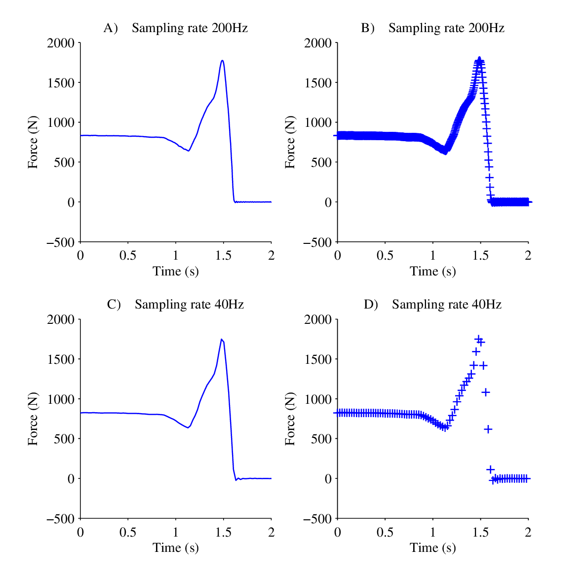
Signals are often shown in figures as continuous lines because when there are many samples in a figure using a symbol for each sample makes the plot look messy like in Figure 1.2 B. It is however important to remember that lines are not actual measured values and just used to connect the dots (if we give each point in a line a value it is called linear interpolation).
If you are plotting the data to inspect if you have sampled often enough it is a good idea to use a symbol to represent each point and leave the lines out. Also make sure you zoom close enough to the closest peaks so you can really tell how far apart successive samples are.
Figure 1.2 shows a the vertical force influencing a force plate while a University lecturer jumps of it. The data was sampled at 200Hz and then decimated to 40Hz using a computer. The lines in subplots A and C look deceptive similar, but subplots B and C suggest that 200Hz is enough to measure the maximum force, but 40Hz is not quite enough and it would be wise to increase the sample rate to be sure. (The difference between maximum forces is 27N).
1.6.1 Random noise and the Gaussian distribution
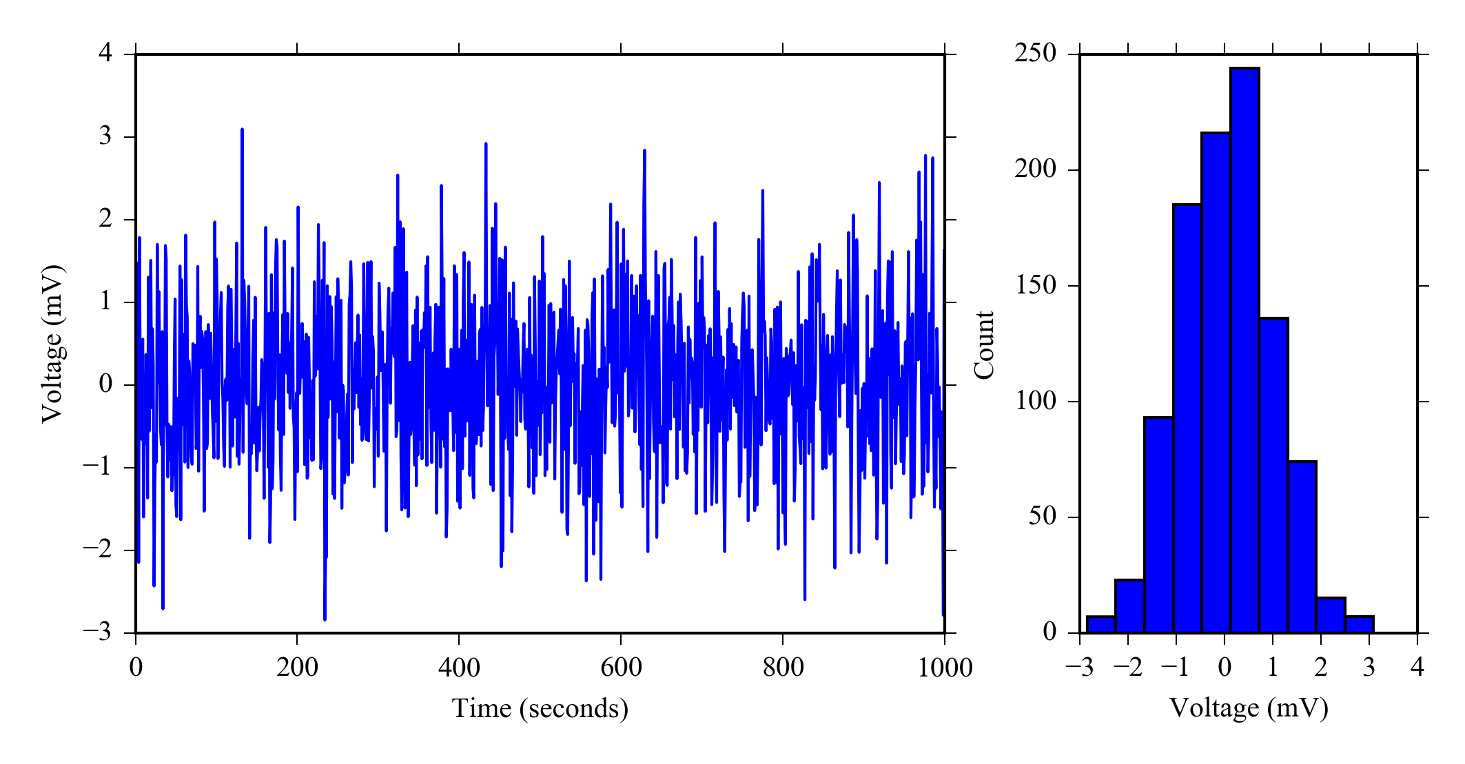
In electronics noise is a random fluctuation in an electrical signal. Random noise has a flat spectral density and a Gaussian distribution . Noise exists in all electronic circuits. Figure 1.3 shows what random noise in a static signal looks like.
Measurements systems generally have noise, fluctuation around the true value. If you only take one sample every 15 minutes the noise level will go unnoticed, however when you take several samples from a sensor at moderately high sample (e.g. 10Hz) there is likely some variability in the values. Although if the noise level in the system is lower than the resolution of your ADC it will be hidden. You can analyze the amount of noise in your system using statistics.
Quantization error is also random noise with a standard deviation of \( \frac{1}{\sqrt{12}} \) LSB. This is usually a small addition to the noise already present in the measured analog signal.
The fact that random noise has a Gaussian distribution means that the the most probable value of the signal is the average value and the standard deviation gives us a meaningful estimate of the variability.
If the signal is stationary during repeated measurements you can make the measured value more precise by taking several samples and averaging. If the signal is not stationary, but the noise is random you can use a moving average filter.
Note that you should check whether or not the noise is Gaussian before you do this. If the signal is not Gaussian then you should check whether the variability in the signal is due to interference and whether or not you can get rid off it by improving the measurement set up or filtering the signal.
The normal distribution (Gaussian) defined as \( N(\mu, \sigma) \) is a bell shaped distribution that has mean \( \mu \) and standard deviation \( \sigma \) .
The parameters can be calculated from sample \( x \) with \( N \) numbers using:
Flat spectral density is another way of saying that the noise doesn’t have a specific frequency that causes more variability than others. You can obtain the spectrogram of the signal using a discrete Fourier transform (DFT), commonly calculated using the FFT algorithm.
Again if there are marked peaks in the spectrum you should try find the origins of those peaks. Power line interference at 50Hz is quite common in measurements, but you can remove it by using a lowpass or band-reject filter. Generally frequency interference can be removed using digital filters (or analog, but digital filters are better).
1.6.2 Measures of signal quality
The following measures can be used to describe the quality of the measured signal:
- Signal-to-noise ratio SNR : is the power ratio between signal and noise. The greater the better.
- Coefficient of variation CV is the inverse of SNR. The smaller the better.
If the signal is normally distributed, then the standard error (SE) or typical error between the mean (from the signal) and the true mean (actual measured value) is given by:
Use at least 10 samples to calculate these, and rather 100 or 1000.
Standard deviation is a measure of precision and you should report it in your results in addition to the mean. Alternatively you can use the standard error.
1.7 Properties of measurements
This section contains brief explanations about the properties of measurements and general terminology. It deals with both static and dynamic measurements.
Static measurement is a measurement of quantity that doesn’t change during sampling e.g. the weight of a Cow at this instant, moisture of grains from a sample from the dryer.
Dynamic measurement is a measurement of constantly chancing quantity and needs additional consideration compared to static measurements. Force measurements of moving objects, speed and acceleration etc.
1.7.1 Accuracy and precision
Suppose you take several static measurements from in a short period of time e.g. measure the weight of a cow several times in a row then:
Accuracy is the difference between the average measured value and correct value. (= bias )
Precision is the variation between the samples i.e. the repeatability of the measurement. It is measured with standard deviation.
Accuracy is a measure of systematic error and precision is a measure of random noise and can be improved using calibration. Precision can be improved by taking more measurements and averaging or in many cases improving the measurement set up.
Note: Accuracy and precision are not synonyms when it comes to technology.
1.7.2 Types of errors
Systematic error : is measured with accuracy
Random error : is measured with precision and can reported using standard deviation or standard error.
Absolute error : magnitude of the difference between the true value and measured value. e.g. absolute error of temperature measurement is \( \pm ^oC \) .
Relative error : is the error in %. \( \frac{\text{absolute error}}{\text{true value}} \cdot 100\% \)
1.7.3 Dynamic properties of measurements
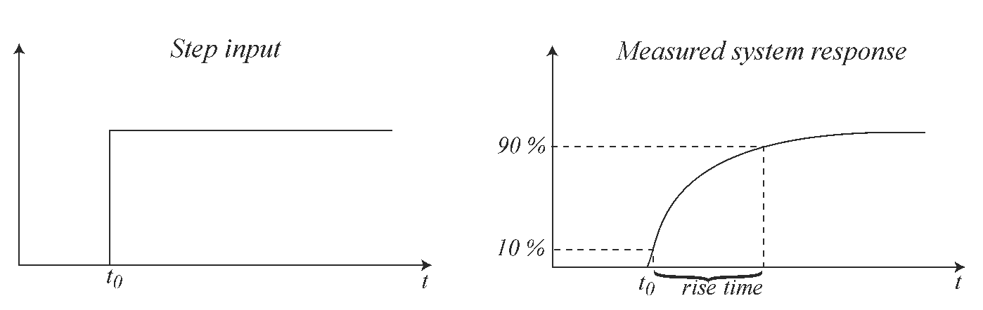
Step response : is the measurement systems response to a step input. It is used to determine the dynamic properties of the system.
1.8 Calibration
In calibration the measured value is compared to the true value (or more accurate value obtained from better instrument or lab analysis).
- Results are used to calculate calibration coefficients .
- Is used to correct systematic error in the measurements.
- It’s important to have enough calibration points, especially if the sensors response curve is not linear.
It usually helps if you know physics you e.g. use a known mass to calibrate force sensors, rotary movement with known radius to calibrate accelerometers, boiling water and ice to calibrate temperature sensors etc. Calibration also needs to be checked during long running measurements because the properties of the sensors or system can change over time. Sensors in tough environments such as cattle buildings or field are especially prone to changes in calibration.
Some instruments have calibration certificates from the manufacturer. There are specialized calibration labs to do the calibration for you.
1.9 More terms
Span : This is the measurement range of an instrument e.g. 0-5 V, -10 – 10V.
Drift: is the change of the zero level of a measurement over time. Drifting can occur e.g. due to temperature when the properties of the amplifiers or sensors change.
Sensitivity is the change in output of the sensor relative to the input: 10 \( \frac{mV}{^o C} \) , \( \frac{mV}{V} \) …
Resolution tells how accurately a quantity can be measured with a sensor or a system. For ADCs the resolution is expressed in bits and you can calculate the voltage resolution. For sensors this is usually indicated in the measured unit e.g. \( \pm 0.1 ^{\circ} \) C or \( \pm 2cm \) .
The sensitivity of a 500kg load cell is 2mV/V f.s. (full scale). With the recommended input voltage 10V the sensitivity is 20mV/500 kg, which means that if we want to measure force with 1 kg resolution we need to be able to measure voltage with 0.04 mV resolution.
Hysteresis means that there is a difference in readings depending whether the measured value is approached from above or below (e.g. rising or falling temperature).
1.10 Exercises
- LM35A is integrated circuit temperature sensor. Answer following questions based on the datasheet:( http://www.ti.com/lit/ds/symlink/lm35.pdf )
- Accuracy
- Measurement range
- Rise time from 0-100% in still air?
- Write the equation for converting LM35 voltage into temperature in \( ^{\circ} \) C.
- What would be a good agricultural application for the sensor?
- The resolution of an ADC is 12bits and the span is 0-5V. What is the voltage resolution?
-
Explain the following terms:
- Hysteresis
- Accuracy
- Sensitivity
- Precision
- Rise time
- Least significant bit
- How do you choose a sampling rate for a dynamic measurement?
- You want to measure weight with 1kg resolution starting from 0kg. What is the maximum weight you can measure with a 12bit ADC?
- How do you measure the rise time of a system?
- What are the advantages of digital signals over analog signals?
- How would you measure the signal-to-noise ratio of a system?
- Define random noise.