Chapter 5 Scientific Python
Python has a collection of scientific libraries that is called the SciPy stack 1 . It consists of powerful data structures to manipulate multidimensional using simple expressions and powerful routines to perform analysis and data manipulation.
The SciPy stack consists of the following Python modules:
-
NumPy. Multidimensional arrays and basic operations -
SciPy. A library for scientific computing which contains functionality for statistics, signal processing, optimization and linear algebra. -
matplotlibfor plotting -
pandasprovides easy to use data structures for data with mixed data types. -
Sympyfor symbolic math -
IPythonfor a rich Python shell -
nosefor testing.
In addition to these libraries the
statsmodels
package for statistics and the
scikit-learn
package for machine learning are very useful.
We will use the following statement to import most important functionality from NumPy, SciPy and matplotlib into main namespace.
from pylab import *
This form is in my opinion easiest to use for beginners. The pylab module imports core components from Numpy, Scipy and matplotlib for easy interactive use. When you get more familiar with Python you can then import only the parts that you need. Bare in mind that there are also other forms that can be used to import modules when you read examples from various sources.
5.1 NumPy arrays
Numpy package contains efficient multidimensional arrays that form the
basics of data manipulation also in Scipy.
The
array
datatype is
the basic type we are using.
It can used in scalar
computations, like adding two arrays elementwise, or
in linear algebra operations.
Numpy has methods for reading data from files to arrays, creating arrays with a certain range and converting other Python sequences to arrays.
The
linspace
command can be used to create a vector between given
and start endpoints with predetermined number of elements and
arange
commands is used to create vector with elements with certain
difference between elements.
Here are some methods to create arrays:
>>> linspace(0, 1 ,5) #Five elements from 0 to 1
array([ 0.  ,  0.25,  0.5 ,  0.75,  1.  ])
>>> arange(0, 2, 0.3) #From 0 to 2 by 0.3
array([ 0. ,  0.3,  0.6,  0.9,  1.2,  1.5,  1.8])
>>> array([3.2, 1, 4]) #From list
array([ 3.2,  1. ,  4. ])
The advantage of arrays is that they can be used in equations easily without looping trough all elements like you would need to do with a list.
Suppose for instance that we have a 12V power source and we want to calculate the power for currents between 0 and 2A. This is given by formula \( P=VI \)
And the solution using Numpy arrays:
>>> V = 12
>>> I = linspace(0, 2, 6)
>>> I
array([ 0. ,  0.4,  0.8,  1.2,  1.6,  2. ])
>>> P = V*I
>>> P
array([  0. ,   4.8,   9.6,  14.4,  19.2,  24. ])
The following table shows for basic operations on arrays. See Numpy refence for complete details http://docs.scipy.org/doc/numpy/reference/ .
| Operation and remarks | Command |
| Creating variables: | a = 1. |
| vector: from 1-10 | a = arange(1. , 11) |
| array | X = array([[3, 2], [4, 1], [6, 3]]) |
| Basic element wise operations * + -/ | 2. + 5.5; a-3; a*b; X/Y |
| Powers | 2**3; a**2; X**10 |
| Square root | sqrt(a) |
| Indexing arrays | b = a[0:5] |
| Multidimensional arrays [row, column] | Y = X[0:2, 2:5] |
| Number of elements | len(x); shape(X) |
| Sum | sum(x); sum(X) |
| by colums | sum(X, 0) |
| by rows | sum(X, 1) |
| Average | mean(x); mean(X) |
| by colums | mean(X, 0) |
| by rows | mean(X, 1) |
| Standard deviation | std(x); std(X) |
| by colums | std(X, 0) |
| by rows | std(X, 1) |
| Cumulative sum | cumsum(x); cumsum(X) |
| by colums | cumsum(X, 0) |
| by rows | cumsum(X, 1) |
| Dot product | dot(a,b); dot(X,Y) |
| Transposing a matrix | transpose(X) |
| Random numbers | rand(100) |
| from Normal distribution | randn(10,10) |
| Delete a variable | del a |
| Help for a command | help(mean); help(std) |
5.1.1 Saving and loading NumPy arrays
Numpy has easy methods for reading and writing numerical data to and from text files.
A simple example:
>>> x = randn(5, 3)
>>> savetxt('data.txt', x)
>>> x2 = loadtxt('data.txt')
>>> x
array([[ 0.57299917,  0.47370978, -2.60736374],
       [ 0.5965621 , -0.85368156,  1.629525  ],
       [ 1.6277449 , -1.07544523, -0.57351649],
       [-2.44221353, -1.2686372 ,  0.14524342],
       [-1.24633481,  1.12646824,  1.00443323]])
>>> x2
array([[ 0.57299917,  0.47370978, -2.60736374],
       [ 0.5965621 , -0.85368156,  1.629525  ],
       [ 1.6277449 , -1.07544523, -0.57351649],
       [-2.44221353, -1.2686372 ,  0.14524342],
       [-1.24633481,  1.12646824,  1.00443323]])
>>> x == x2
array([[ True,  True,  True],
       [ True,  True,  True],
       [ True,  True,  True],
       [ True,  True,  True],
       [ True,  True,  True]], dtype=bool)
You can also use converters to read in e.g. dates. The following example will load a datafile with dates in the first column and convert the iso formatted date to numeric format.
from matplotlib.dates import datestr2num
data = loadtxt("data.txt", converters = {0: datestr2num})
5.2 pandas dataframes
NumPy arrays are very useful and efficient when you only have numerical data, but they are a lot less convenient to work with when you have data consisting of multiple data types such as strings, factors and booleans. The pandas library provides data structures and functions that make working with mixed data types a lot easier. The library is very well documented at http://pandas.pydata.org , but I will show few examples to give an idea about how the library can be used.
The main pandas data structure is the DataFrame. The library provides a several functions to read a DataFrame from files (csv, excel, hdf5) or from SQL database. You can also construct DataFrames from several data structures e.g. lists, dicts and NumPy arrays.
Here is a simple example about making a DataFrame from a list of Python dicts:
>>> import pandas as pd
>>> cowList = [{"id" : 101, "weight" : 650},
...            {"id" : 102, "weight" : 720},
...            {"id" : 103, "weight" : 800},
...            {"id" : 104, "weight" : 560}]
...
>>> #Create DataFrame
>>> df = pd.DataFrame(cowList)
>>>
>>> #Look at the contents
>>> df
    id  weight
0  101     650
1  102     720
2  103     800
3  104     560
Let’s look at a more interesting example of roughage intake data from dairy cows in feedintake.csv file. The dataset contains roughage feeder trough visit information from 48 cows during 24 hours. Each row corresponds to one visit from a cow with recorded trough number, start and end time, visit duration in seconds and feed intake in kilograms.
We will read the data from csv file using pandas:
>>> feed = pd.read_csv("data/feed_intake.csv")
>>> #Look at the first rows using head function
>>> feed.head()
   cowID  trough                begin                  end  duration  intake
0      9      18  2015-08-18 00:03:50  2015-08-18 00:12:03       493     2.5
1      2      13  2015-08-18 00:06:27  2015-08-18 00:12:18       351     1.3
2      9      18  2015-08-18 00:12:32  2015-08-18 00:17:51       319     1.3
3     43      11  2015-08-18 00:08:06  2015-08-18 00:20:09       723     3.5
4     42      23  2015-08-18 00:03:38  2015-08-18 00:21:10      1052     4.6
We can access the columns of the DataFrame with the column name:
>>> feed["intake"].head()
0    2.5
1    1.3
2    1.3
3    3.5
4    4.6
Name: intake, dtype: float64
>>> feed["duration"].head()
0     493
1     351
2     319
3     723
4    1052
Name: duration, dtype: int64
And also remove columns, note that the inplace option can be used to modify an existing object and is more efficient.
# Make a copy with dropped column
feed2 = feed.drop(["trough"], 1)
# Modify existing object
feed.drop(["trough"], 1, inplace =True)
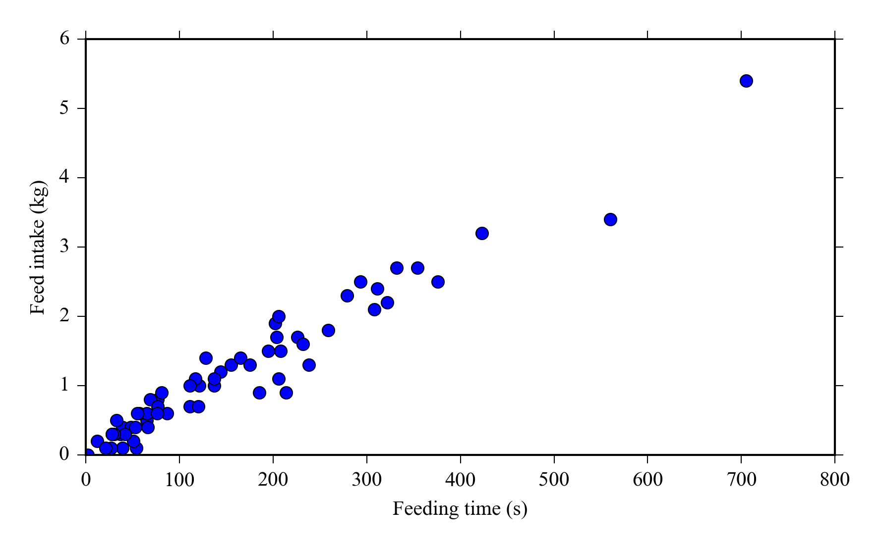
And select data from the DataFrame e.g. select all data from cow number 1 and plot feed intake vs feeding bout duration:
cow1 = feed[feed["cowID"] == 1]
plot(cow1["duration"], cow1["intake"], 'o')
xlabel("Feeding time (s)")
ylabel("Feed intake (kg)")
We can easily calculate the total feed intake and feeding time for each cow by grouping the dataset by “cowID” column and applying the sum function.
>>> feed_sums = feed.groupby("cowID").sum()
>>> feed_sums.head()
       duration  intake
cowID
1          9778    73.6
2         11868    66.0
3           858     2.4
4          9796    68.8
5         12848    69.7
You can also apply several aggregate function passing them as a list
>>> feed.groupby("cowID").agg([np.sum, np.std]).head()
      duration             intake
           sum         std    sum       std
cowID
1         9778  136.811512   73.6  0.995150
2        11868  235.607678   66.0  1.480723
3          858  109.874474    2.4  0.551362
4         9796  491.439436   68.8  3.548356
5        12848  227.878629   69.7  1.546469